The analysis of optimization in music aesthetic education under artificial intelligence

The combination of AI and music aesthetic education

AI is a science and technology field dedicated to understanding and creating intelligent behaviors. AI integrates the knowledge of computer science, statistics, cognitive science and other disciplines, aiming at researching, designing and developing intelligent agents. These agents can perceive the environment, learn, reason, solve problems and make decisions independently. The application forms of AI are diverse, covering but not limited to robotics, speech recognition, image recognition, natural language processing (NLP), expert system and machine learning. According to its function and complexity, AI can be further divided into three levels: weak AI, strong AI and super AI¹⁸. Its hierarchical division is shown in Fig. 1 below:

Weak AI focuses on and is good at the performance of specific tasks. While strong AI has cross-disciplinary and comprehensive human-level intelligence and can perform any cognitive task that human beings can complete. As for strong AI, it is assumed that it exists beyond the limits of human intelligence and can be far superior to the best human beings in all cognitive abilities^12,15,19. With the development of technology, AI is increasingly infiltrating into all aspects of social life, and continues to promote scientific and technological progress and industrial upgrading²⁰.

With the continuous development of AI technology, reshaping music provides more support and creativity for cultivating students’ academic accomplishment, aesthetic perception, artistic expression and cultural understanding. On this basis, the possibility of using AI technology to promote the reform and development of music aesthetic teaching is discussed^21,22. By applying advanced AI technology, music aesthetic education can realize more refined and personalized teaching strategies. The relationship between them is shown in Table 1:

On one hand, AI can accurately identify and assess students’ musical aesthetic tendencies, learning styles, and ability levels through big data analysis and algorithmic models. This enables the provision of personalized teaching content and learning paths, enhancing the relevance and effectiveness of teaching. On the other hand, AI can also be employed in emotional analysis, style identification, creative assistance, and other aspects of music composition. This aids students in gaining a deeper understanding of the internal structure and external expression of music, thereby broadening their aesthetic horizons and enhancing their appreciation of music. Furthermore, intelligent music teaching systems can facilitate students’ active engagement and immersive learning experiences through real-time feedback and interaction. This shift from traditional indoctrination to a new teaching mode focused on inquiry and experiential learning promotes both the quality and efficiency of music aesthetic education, leading to a dual improvement in educational outcomes²³.

DL algorithm

DL is a machine learning method, which is inspired by the working principle of human brain neural network, and carries out high-level abstraction and learning of data by constructing a series of interconnected artificial neural network (ANN) levels²⁴. In the DL model, the original input (such as image pixels, text characters or sound waveforms) first passes through a multi-level nonlinear transformation. Each layer will extract more and more complex feature representations from the input data. This layer-by-layer processing mechanism enables the model to automatically learn and explore useful features from the original data without artificially designing features^25,26,27. The core technologies of DL include deep neural networks (such as convolutional neural networks, recurrent neural networks, long and short-term memory networks, etc.). They are excellent in solving many complex problems such as image recognition, speech recognition, NLP, machine translation, recommendation system, game strategy, and automatic driving. By updating model parameters through optimization algorithms (such as back propagation algorithm), the DL model can self-train and improve on large-scale datasets, thus achieving high-precision prediction and decision-making ability²⁸. With the enhancement of computing power and the popularity of big data, DL has become one of the key technologies in the field of modern AI and has made revolutionary breakthroughs in many industries²⁹.

The unsupervised learning algorithm of DL can be used to learn the intrinsic feature representation of music signals. By employing dimensionality reduction and reconstructing music data, self-encoders are capable of extracting meaningful music features from the original audio signal. These features may include rhythm, timbre, and harmonic structure, among others. Such extracted features can aid teachers in designing and implementing targeted teaching activities³⁰. A typical unsupervised learning method is to find the “best” representation for data. “Best” can be articulated differently, but it typically implies certain constraints or limitations compared to the information it inherently conveys. In essence, it signifies having fewer advantages or constraints. Therefore, it is essential to retain as much information about X as possible.

The matrix X is designed as a combination of \(m \times n\). The average value of the data is 0, that is, \(E\left[ x \right]=0\). If it is not 0, the average value is subtracted from all samples in the preprocessing step, and the data is easily centralized³¹. The unbiased sample covariance matrix corresponding to X is given as follows:

Var[z] is a diagonal matrix which is transformed into z=\(\:{W}^{T}x\) by linear transformation. The principal component of the design matrix X is given by the eigenvector of \({X^T}X\)³², as follows:

Assume that W is the right singular vector of singular value decomposition \(X=U\sum {{W^T}} \), and taking W as the basis of eigenvector, the original eigenvalue equation can be obtained as follows:

This can fully explain that Var[z] in the algorithm is a diagonal matrix. Using the principal component decomposition of X, the variance of X can be expressed as:

\({U^T}U=I\) is used, because the matrix U is orthogonal according to the definition of singular value, which shows that the covariance of z meets the diagonal requirements, as shown below:

The above analysis shows that when the data x is projected to z through linear transformation w. The covariance matrix represented by the obtained data is diagonal \(\left( {\sum {^{2}} } \right)\), which means that the elements in Z are independent of each other¹.

Through these unsupervised learning techniques, music aesthetic education can become more intelligent and personalized. Meanwhile, it can help teachers and researchers to examine and optimize teaching methods from a new perspective, thus improving the quality and effect of music education.

Music aesthetic education method based on DL in AI environment

On this basis, this paper puts forward a new music aesthetic teaching mode based on DL. Based on AI, the system provides various supporting services for students’ learning^33,34. The functional design of the system is shown in Fig. 2:

The role of machine learning in the music industry is to extract “data” from a piece of music, input it into a specific pattern, learn “features” from it, and analyze and sort it out. The specific pseudo code is arranged as follows:

Initialize AI model with multimodal deep learning framework.

Input music features (MFCC, PLP, melody) and emotional data (Arousal, Valence).

Train and optimize model for personalized music aesthetic education feedback.

With the help of DL technology, AI can deeply understand each student’s learning style, interest tendency and skill level through the analysis of a large number of user data. Then, AI provides customized music appreciation and learning content. The purpose is to ensure that music aesthetic education meets individual needs more accurately and truly teach students in accordance with their aptitude³⁵. Meanwhile, AI can monitor and respond to students’ learning behavior and feedback in real time. It can dynamically adjust the teaching plan to ensure that the educational process is efficient and targeted, thereby enhancing the effectiveness of the learning experience. Secondly, DL strengthens the interactive experience in music education. By integrating VR/AR technology and DL algorithm, a highly immersive music teaching environment is constructed, so that students can directly feel the rhythm, melody, harmony and other aesthetic elements in music works in VR.

Music features and music emotion model based on DL in AI environment

The musical features studied here are mainly divided into Mel-frequency cepstral coefficient (MFCC) features and Perceptual Linear Prediction (PLP) features. Two kinds: MFCC is a feature parameter widely used in speech signal processing, especially in speech recognition and speaker recognition. The core idea of MFCC is to simulate the sound perception mechanism of human auditory system. PLP feature is also a feature parameter commonly used in speech recognition, but unlike MFCC, PLP feature is more directly based on human auditory perception model. PLP enhances speech recognition through a series of auditory perception simulations of speech signal spectrum.

The musical emotion model in this paper is Long Short-Term Memory (LSTM) model. LSTM is a variant of RNN and one of the important components of the neural network model designed and constructed in this paper. LSTM not only inherits the advantages of traditional RNN, but also overcomes the problem of gradient explosion or disappearance of RNN. It can effectively process arbitrary length series data and capture long-term dependence of data, and the total amount of data processed and training speed have been greatly improved compared with traditional machine learning models. LSTM consists of many repeating units, which are called memory blocks. Each memory block contains three gates and one memory unit, and the three gates are forget gate, input gate and output gate respectively. The specific calculation flow of the memory block is shown in Fig. 3:

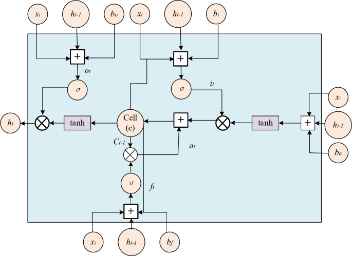
Network structure diagram of LSTM.

The equation for calculating the input layer information for obtaining the upper input unit data is as follows:

\({v_t}\): The value of the candidate memory cell.

\(\tanh \): Hyperbolic tangent activation function, which is used to compress the input into [-1, 1] interval.

\({w_{xa}}\): The weight input to the candidate memory unit.

\({w_{ha}}\): Weight of hidden state to candidate memory cells at the previous moment.

\({x_t}\): Input at the current moment.

\({h_{t – 1}}\): The hidden state of the previous moment.

\({b_a}\): Bias of candidate memory cells.

Input gate, forget gate and output gate are controlled by Sigmoid function, and the specific calculation equation is as follows:

\({i_t}\): Input the activation value of the gate to control the degree to which the current input information enters the memory unit.

σ: Sigmoid activates the function, which compresses the input into the interval of [0, 1] and is used to control the flow of information.

\({w_{xi}}\): The weight input to the input gate.

\({w_{hi}}\): The weight of the hidden state to the input gate at the previous moment.

\({b_i}\): Offset of input gate.

\({f_t}\): The activation value of the forgetting gate controls the degree of information retention of the memory cell at the previous moment.

\({w_{xf}}\): The weight entered the forget gate.

\({w_{hf}}\): The weight from the hidden state to the forgotten gate at the previous moment.

\({b_f}\): Offset of forget gate.

\({o_t}\): The activation value of the output gate controls the information output degree of the memory unit at the current moment.

\({w_{x0}}\): The weight input to the output gate.

\({w_{h0}}\): The weight of the hidden state to the output gate at the previous moment.

\({b_0}\): Offset of output gate.

σ represents Sigmoid function, and the calculation equation is:

The state values of the memory cell and the output gate are calculated as follows:

\({c_t}\): Memory cell state at the current moment.

\( \odot \): Multiplication at the element level (Hadamard product).

\({c_{t – 1}}\): The state of the memory cell at the previous moment.

\({a_t}\): Candidate memory cell states at the current moment.

\({h_t}\): The hidden state of the current moment.

\(\tanh ({c_t})\): Apply hyperbolic tangent activation function to the memory cell state at the current moment.